Engineering Economics
Compare designs by the value they deliver over their useful lives.
The least expensive purchase can cost more
A design decision includes acquisition, installation, energy, consumables, maintenance, downtime, and end-of-life effects. Compare alternatives on an equivalent service basis, with a shared study period and explicit assumptions.
Present worth
For initial cost \(C_0\), annual net benefits \(B_t\), terminal salvage value \(S\), discount rate \(i\), and study period \(n\):
\[NPV=-C_0+\sum_{t=1}^{n}\frac{B_t}{(1+i)^t}+\frac{S}{(1+i)^n}.\]
For cost-only alternatives, compare discounted lifecycle costs and select the lowest feasible cost under the stated assumptions. For mutually exclusive projects with benefits, compare incremental cash flows and constraints rather than selecting solely by percentage return.
Try a simple design investment
This calculator assumes a year-zero investment, equal net benefits at each year-end, and terminal salvage. Cash flows and discount rate must use a consistent real or nominal basis. It omits taxes, financing, and inflation adjustments.
At the default inputs, NPV is approximately $7,296. A positive result means the modeled benefits exceed modeled costs at the chosen discount rate; it does not prove that the design is safe, feasible, or the best alternative.
Eight cash-flow factor calculators
Use these calculators for the eight cases on the reference sheet. Each one calculates an equivalence at a selected rate; it does not predict investment returns.
- P: present amount at time 0. F: future amount at the end of period n.
- A: equal payment at the end of every period, from 1 through n.
- G: increase per period in an arithmetic gradient, with zero gradient in period 1.
- i: effective interest or discount rate per period, entered below as a percentage. n: number of periods.
Match the units. For annual cash flows, use an effective annual rate and years. For monthly cash flows, use an effective monthly rate and months. An 8% effective annual rate converts to a monthly rate of 100 × ((1.08)^(1/12) − 1) percent; a nominal annual rate compounded monthly is divided by 12. Beginning-of-period payments require different timing adjustments.
How to read the diagrams: The green upper row shows the known cash-flow pattern; the gold lower row shows the equivalent pattern being calculated. Both rows depict positive amounts for comparison. They are alternative representations, not two sets of payments to add together. Actual inflows and outflows use signs consistent with your viewpoint. Each illustration uses five periods and schematic arrow heights; it stays fixed when calculator inputs change. The expandable cash-flow schedule below each calculator reflects the entered values.
All examples start at 8% for 5 periods. These calculators support rates from 0% to 100% per period and whole-number periods from 1 to 200. Amounts may be signed; keep inflows and outflows consistent. Results use unrounded factors internally. Taxes, inflation, fees, and changing rates are excluded.
Single payment: compound amount
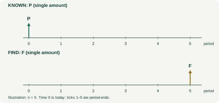
Reading the graphic: The upper timeline places the known amount P at time 0. The lower timeline replaces it with one equivalent amount F at the end of period 5. Moving forward in time means multiplying by (1 + i) once per period, so the exponent n counts the full intervals between the two amounts. There are no intermediate deposits in this case. At the default inputs, $10,000 today becomes $14,693.28 after five years at 8% per year.
Find the future value of one amount invested today. P is at time 0; F is at the end of period n.
Example: A $10,000 machine-replacement reserve earns 8% per year for 5 years. How much is available at the end?
Single payment: present worth
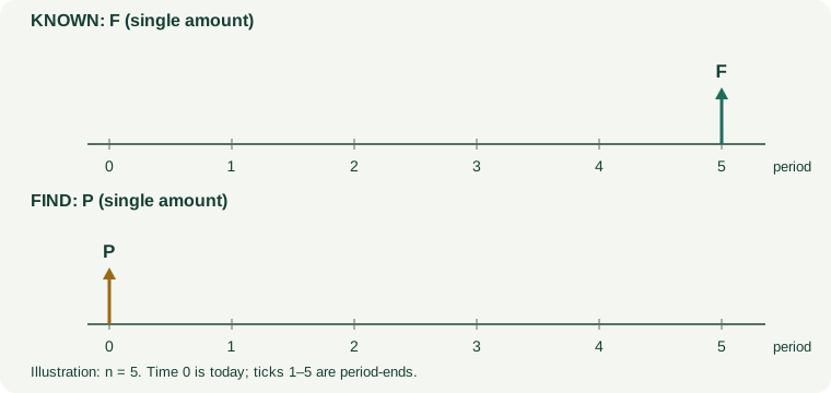
Reading the graphic: The known future amount F appears at the last tick on the upper timeline. The lower timeline shows its equivalent P today, at time 0. Moving backward through n periods means dividing by (1 + i) to the nth power. With a positive discount rate, the present equivalent of a positive future amount is smaller. At the default inputs, $10,000 due in five years has a present equivalent of $6,805.83 at 8% per year.
Find the amount needed today to equal a specified future amount at the chosen rate. Discount one payment from period n back to time 0.
Example: A replacement will cost $10,000 in 5 years. What is its present equivalent at 8% per year?
Uniform series: compound amount
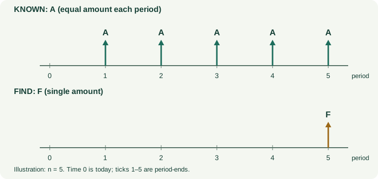
Reading the graphic: Each A arrow on the upper timeline is the same amount, paid at the end of periods 1 through 5. There is no payment at time 0. The single F arrow below is the accumulated value immediately after the last payment. The first A earns interest for n - 1 periods; the last A earns none before the valuation. The F/A factor adds these differently compounded amounts. Five year-end deposits of $1,000 at 8% accumulate to $5,866.60.
Find the future value of equal end-of-period deposits. There are n deposits, beginning at period 1; the final deposit is included at period n and earns no interest before that valuation.
Example: Deposit $1,000 at each year-end for 5 years at 8%. Find the accumulated reserve just after the fifth deposit.
Uniform series: sinking fund
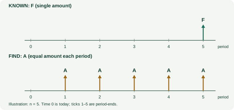
Reading the graphic: The upper timeline shows the known future target F. The lower timeline asks for the same deposit A at each period-end, including period 5. Earlier deposits earn interest for longer, so at a positive rate the required A is less than F/n. This is the inverse of the F/A calculation. To reach $10,000 at the end of five years at 8%, deposit $1,704.56 at each year-end; the displayed cents are rounded.
Find the equal end-of-period deposit needed to reach a future target. There is no initial deposit at time 0.
Example: Build a $10,000 replacement fund in 5 years at 8%. How much should be deposited each year-end?
Uniform series: capital recovery
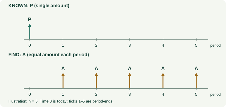
Reading the graphic: The upper timeline places the amount to be recovered or financed at time 0. The five A arrows below represent an equivalent level payment stream beginning one period later. The A/P factor recovers the principal and accounts for the chosen rate; at a positive rate, A exceeds P/n. A $10,000 amount financed at 8% over five annual payments gives $2,504.56 per year before fees. For an actual borrower transaction, the initial loan receipt and repayments have opposite signs; these paired diagrams show equivalence of magnitudes.
Convert a present amount into n equivalent equal end-of-period payments. This includes recovery of the principal and the return represented by i. A loan example assumes no fees and a fixed periodic rate.
Example: Finance a $10,000 machine over 5 years at 8% per year. Find the equal annual payment.
Uniform series: present worth
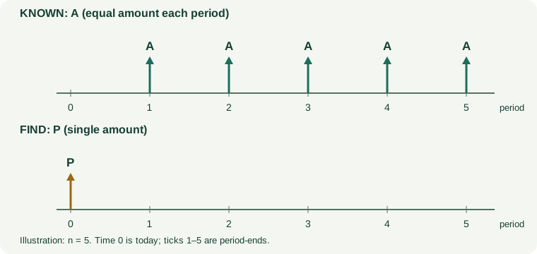
Reading the graphic: The five equal A arrows above occur at periods 1 through 5. Each is discounted separately to the time-0 P arrow below: the first payment travels back one period and the final payment travels back five. The P/A factor adds those discounted values. Because later payments are discounted more heavily, the result is less than nA when the rate is positive. Five annual savings of $1,000 have a present equivalent of $3,992.71 at 8%.
Find the present equivalent of n equal end-of-period payments. The first payment occurs one period from today.
Example: A design saves $1,000 at each year-end for 5 years. What are those savings worth today at an 8% discount rate?
Arithmetic gradient: uniform series
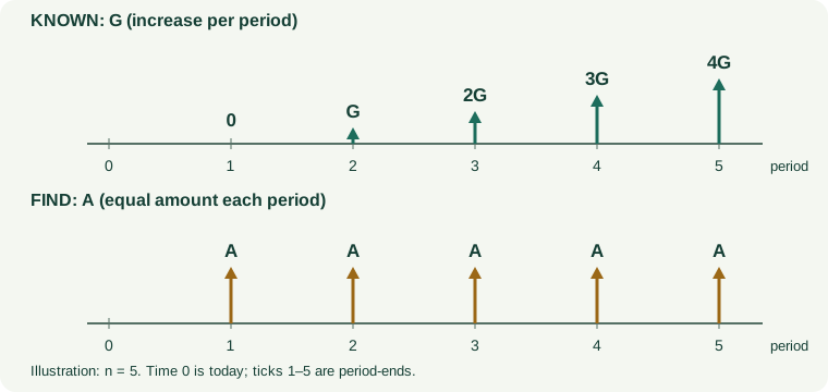
Reading the graphic: Read the upper timeline carefully: the gradient portion is zero at period 1, then G at period 2, 2G at period 3, and finally 4G at period 5. The lower timeline spreads its economic equivalent into five equal amounts A, including a payment in period 1. This is a discounted equivalence, not simply an arithmetic average at a positive rate. For G = $1,000 and i = 8%, the equivalent annual amount is $1,846.47. If there is also a constant base amount B every period, add B to this result.
Convert a cash-flow increase of G per period into an equivalent constant end-of-period amount. The gradient alone is 0, G, 2G, …, (n − 1)G in periods 1 through n.
Example: Extra maintenance is $0, $1,000, $2,000, $3,000, and $4,000 at the ends of years 1–5. Find its equivalent annual cost at 8%.
Arithmetic gradient: present worth
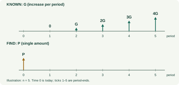
Reading the graphic: The increasing arrows above represent the gradient portion only. Its zero at period 1 is one period after today; it must not be mistaken for time 0. The first nonzero amount G occurs at period 2. The P/G factor discounts each increasing amount from its own period to the single P arrow below. For five periods with G = $1,000 and i = 8%, the present equivalent is $7,372.43. If the actual costs start with a base amount B in period 1, add B times the P/A factor for the same i and n.
Find the time-0 equivalent of a cash-flow increase of G each period. Period 1 has zero gradient; the first G occurs at the end of period 2.
Example: Discount extra maintenance of $0, $1,000, $2,000, $3,000, and $4,000 in years 1–5 to time 0 at 8%.
Add uncertainty to the decision
Estimate optimistic, expected, and adverse scenarios. Vary utilization, energy prices, maintenance, and service life separately, then consider combinations. Find the break-even annual benefit. Present the assumptions that could reverse the recommendation.
Simple payback is initial investment divided by constant annual net benefit. It is easy to communicate but ignores discounting and cash flows after payback. Use it as a supplementary measure.
A reproducible R example
initial <- 30000
benefit <- 9000
years <- 5
rate <- 0.08
salvage <- 2000
npv <- -initial + sum(benefit / (1 + rate)^(1:years)) +
  salvage / (1 + rate)^years
round(npv, 2)
The same example in MATLAB
This version uses the same year-zero investment, five equal year-end net benefits, and salvage received at the end of year 5. MATLAB’s .^ and ./ operators apply the discounting element by element across the vector of years.
initial = 30000;
benefit = 9000;
years = 5;
rate = 0.08;
salvage = 2000;

t = 1:years;
npv = -initial + sum(benefit ./ (1 + rate).^t) ...
    + salvage / (1 + rate)^years;
fprintf('Net present value: $%.2f\n', npv);
The same example in Python
This version uses only built-in Python features. range(1, years + 1) includes years 1 through 5, and ** means exponentiation. The generator inside sum() discounts each year-end benefit separately.
initial = 30000
benefit = 9000
years = 5
rate = 0.08
salvage = 2000

npv = (
    -initial
    + sum(benefit / (1 + rate) ** t
          for t in range(1, years + 1))
    + salvage / (1 + rate) ** years
)
print(f"Net present value: ${npv:.2f}")
All three versions calculate the same net present value: $7,295.56. The negative initial investment occurs at time 0, so it is not discounted. Each annual benefit is discounted from its own year-end, and the salvage is added to the final year’s benefit before considering its present equivalent. Keep the cash flows and discount rate on a consistent real or nominal basis; the examples omit taxes, financing, and inflation adjustments.
What belongs in a senior design report?
Include a bill of materials, cost sources and dates, recurring expenses, study period, discount-rate rationale, economic comparison, and sensitivity analysis. Identify nonmonetary requirements—particularly safety and accessibility—that cannot be traded away simply because an alternative has a favorable NPV.